Overview

This is my note for Chapter 1 of Reinforcement Learning Theory.

Markov Decision Process

Discounted (Infinite-Horizon) MDP

• $\mathcal{S}$$\mathcal{S}$ finite or countably infinite

• $\mathcal{A}$$\mathcal{A}$ finite

• $P$$P$ transition function (conditional distribution for state), where $P(s^{\prime }|s,a)$$P(s' | s, a)$ is the probability of transitioning into $s^{\prime }$$s'$ given $s$$s$ and $a$$a$. Note that $P_{s,a}$$P_{s,a}$ denotes $P(\cdot |s,a)$$P(\cdot| s, a)$.

• $r$$r$ bounded in $[0,1]$$[0,1]$. Deterministic unless specified.

• $\gamma$$\gamma$ bounded in $[0,1)$$[0, 1)$, which defines a horizon.

  • Remarks: 1. This is why it is called discounted MDP. 2. I assume it works like how eigenvalue defines the smoothness for an RKHS?

• $\mu$$\mu$ is an initial state distribution.

objective, policies, and values

• trajectory ${\tau }_t=(s_0,a_0,r_0,s_1,\dots ,s_t,a_t,r_t)$$\tau_t=(s_0,a_0,r_0,s_1,\dots,s_t,a_t,r_t)$

  • Remarks: 1. It goes like state->action->reward->state->..., and each state is a sample. 2. Sort of like a filtration for a stochastic process

• policy $\pi$$\pi$ is a mapping: $\mathcal{H}\to \mathrm{\Delta }(\mathcal{A})$$\mathcal{H}\to\Delta(\mathcal{A})$. A stationary policy mapping $\pi :\mathcal{S}\to \mathrm{\Delta }(\mathcal{A})$$\pi:\mathcal{S}\to\Delta(\mathcal{A})$. A deterministic, stationary policy mapping $\pi :\mathcal{S}\to \mathcal{A}$$\pi:\mathcal{S}\to\mathcal{A}$.

  • Remarks: 1. $a_t\sim \pi (\cdot |{\tau }_{t-1},s_t)$$a_t\sim \pi(\cdot|\tau_{t-1}, s_t)$? sort of weird

• value $V_M^{\pi }:\mathcal{S}\to \mathbb{R}$$V_M^\pi:\mathcal{S} \to \mathbb{R}$ is defined as:

  $$V_M^{\pi }(s)=\mathbb{E}[\sum _{t=0}^{\mathrm{\infty }}{\gamma }^{t}r(s_t,a_t)|\pi ,s_0=s],$$

  which is bounded by $1/(1-\gamma )$$1 / (1- \gamma)$.

• Similarly, action-value (Q-value) $Q_M^{\pi }:\mathcal{S}\times \mathcal{A}\to \mathbb{R}$$Q_M^\pi:\mathcal{S}\times\mathcal{A}\to\mathbb{R}$​ is defined as

  $$Q_M^{\pi }(s,a)=\mathbb{E}[\sum _{t=0}^{\mathrm{\infty }}{\gamma }^{t}r(s_t,a_t)|\pi ,s_0=s,a_0=a],$$

  which is also bounded by $1/(1-\gamma )$$1 / (1- \gamma)$.

• Goal: find optimal policy given starting state $s$$s$:

  $$\underset{\pi }{max}{V}_M^{\pi }(s)$$

Bellman Consistency Equations for Stationary Policies

Lemma 1.4. Suppose that $\pi$$\pi$ is a stationary policy. Then $V^{\pi }$$V^\pi$ and $Q^{\pi }$$Q^\pi$ satisfy the following Bellman consistency equations: for all $s\in \mathcal{S},a\in \mathcal{A},$$s\in\mathcal{S},a\in\mathcal{A},$

Proof:

It is helpful to view $V^{\pi }$$V^\pi$ as vector of length $|\mathcal{S}|$$|\mathcal S|$ and $Q^{\pi }$$Q^\pi$ and $r$$r$ as vectors of length $|\mathcal{S}|·|\mathcal{A}|$$|\mathcal S|·|\mathcal A|$. We overload notation and let $P$$P$ also refer to a matrix of size $(|\mathcal{S}|\cdot |\mathcal{A}|)\times |\mathcal{S}|$$(|\mathcal S|\cdot|\mathcal A|)\times|\mathcal S|$ where the entry $P_{(s,a),s^{\prime }}$$P_{(s,a),s'}$ is equal to $P(s^{\prime }|s,a)$$P(s'|s,a)$.

Remarks: This is straightforward since a function is in some sense an infinite dimensional vector where each point is a coordinate.

We also will define $P^{\pi }$$P^{\pi}$ to be the transition matrix on state-action pairs induced by a stationary policy $\pi$$\pi$, specifically

Remarks: $P^{\pi }\in {\mathbb{R}}^{(|\mathcal{S}|\cdot |\mathcal{A}|)\times (|\mathcal{S}|\cdot |\mathcal{A}|)}$$P^\pi \in \mathbb R^{(|\mathcal S|\cdot|\mathcal A|)\times(|\mathcal S|\cdot|\mathcal A|)}$

In particular, for deterministic policies, we have:

With this notation, it is straightforward to verify

Proof: Notice that

Thus, we have

Also, note that

Corollary 1.5. Suppose that $\pi$$\pi$ is a stationary policy. We have that.

where $I$$I$ is the identity matrix.

Proof: we need to show that $I-\gamma P^{\pi }$$I - \gamma P^\pi$ is invertible, which is to show that for all non-zero vector $x$$x$, $(I-\gamma P^{\pi })x\ne 0$$(I - \gamma P^\pi)x \ne 0$.

To see that the $I-\gamma P^{\pi }$$I-\gamma P^\pi$ is invertible, observe that for any non-zero vector $x\in {\mathbb{R}}^{|\mathcal{S}||\mathcal{A}|}$$x\in\mathbb{R}^{|\mathcal{S}||\mathcal{A}|}$

which implies $I-\gamma P^{\pi }$$I-\gamma P^\pi$ is full rank.

Lemma 1.6. We have that

so we can view the $(s,a)$$(s,a)$-th row of this matrix as an induced distribution over states and actions when following $\pi$$\pi$ after starting with $s_0=s$$s_0=s$ and $a_0=a$$a_0=a$

Proof: we need to show $\sum _{t=0}^{\mathrm{\infty }}{\gamma }^t{\mathbb{P}}_t^{\pi }(I-\gamma P^{\pi })=I$$\sum_{t=0}^{\infty} \gamma^t \mathbb{P}_t^\pi (I-\gamma P^\pi) = I$, where we use ${\mathbb{P}}_t^{\pi }$$\mathbb{P}_t^\pi$ to denote the transition matrix where $[{\mathbb{P}}_t^{\pi }{]}_{(s,a),(s^{\prime },a^{\prime })}={\mathbb{P}}^{\pi }(s_t=s^{\prime },a_t=a^{\prime }|s_0=s,a_0=a)$$[\mathbb{P}_t^\pi]_{(s, a), (s', a')} = \mathbb P^\pi(s_t=s',a_t=a'|s_0=s,a_0=a)$.

Thus, for the element at $(s,a),(s^{″},a^{″})$$(s, a), (s'', a'')$, we need to show

For the LHS, we have

where in the second equation we use the Chapman-Kolmogorov equation. Thus the proof is completed by that ${\mathbb{P}}^{\pi }(s_0=s^{″},a_0=a^{″}|s_0=s,a_0=a)=\mathbb{I}\{(s,a)=(s^{″},a^{″})\}$$\mathbb P^\pi(s_0=s'',a_{0}=a''|s_0=s,a_0=a) = \mathbb{I}\{(s, a)=(s'',a'')\}$.

Bellman Optimality Equations

There exists a stationary and deterministic policy that simultaneously maximizes $V^{\pi }(s)$$V^\pi(s)$ for all $s$$s$.

Theorem 1.7. Let $\mathrm{\Pi }$$\Pi$ be the set of all non-stationary and randomized policies. Define

which is finite since $V^{\pi }(s)$$V^{\pi}(s)$ and $Q^{\pi }(s,a)$$Q^{\pi}(s,a)$ are bounded between 0 and $1/(1-\gamma )$$1/(1-\gamma)$.

There exists a stationary and deterministic policy $\pi$$\pi$ such that for all $s\in \mathcal{S}$$s\in\mathcal{S}$ and $a\in \mathcal{A},$$a\in\mathcal{A},$

We refer to such a $\pi$$\pi$ as an optimal policy.

Proof at P9 of the book.

Remarks: The optimal policy used in the proof is $\tilde{\pi }(s)=\arg \underset{a\in \mathcal{A}}{sup}\mathbb{E}[r(s,a)+\gamma V^{\star }(s_1)|(S_0,A_0)=(s,a)]$$\widetilde{\pi}(s)=\arg \sup\limits_{a\in \mathcal A}\mathbb{E}[r(s,a)+\gamma V^{\star}(s_1)|(S_0,A_0)=(s,a)]$.

Theorem 1.8 (Bellman optimality equations). We say that a vector $Q\in {\mathbb{R}}^{|\mathcal{S}||\mathcal{A}|}$$Q \in \mathbb{R}^{|\mathcal{S}||\mathcal{A}|}$ satisfies the Bellman optimality equations if:

For any $Q\in {\mathbb{R}}^{|\mathcal{S}||\mathcal{A}|},$$Q\in\mathbb{R}^{|\mathcal{S}||\mathcal{A}|},$ we have that $Q=Q^{\star }$$Q=Q^\star$ if and only if $Q$$Q$ satisfies the Bellman optimality equations. Furthermore, the deterministic policy defined by $\pi (s)\in {\mathrm{argmax}}_{a\in \mathcal{A}}{Q}^{\star }(s,a)$$\pi(s)\in\operatorname{argmax}_{a\in\mathcal{A}}Q^{\star}(s,a)$ is an optimal policy (where ties are broken in some arbitrary manner).

Proof at P10 of the book.

Notice that $V^{\ast }(s)=V^{{\pi }^{\ast }}(s)=Q^{{\pi }^{\ast }}(s,{\pi }^{\ast }(s))\ge Q(s,a)(\mathrm{\forall }a)$$V^*(s) = V^{\pi^*}(s) = Q^{\pi^*}(s, \pi^*(s)) \ge Q(s, a) \quad(\forall a)$, when ${\pi }^{\ast }$$\pi^*$ is the optimal stationary and deterministic policy.

Remarks: Here more notations are introduced:

• greedy policy: ${\pi }_Q(s):={\mathrm{argmax}}_{a\in \mathcal{A}}Q(s,a)$$\pi_Q(s):=\operatorname{argmax}_{a\in\mathcal{A}}Q(s,a)$ with respect to a vector $Q\in {\mathbb{R}}^{|\mathcal{S}||\mathcal{A}|}$$Q\in\mathbb{R}^{|\mathcal{S}||{\mathcal{A}}|}$. (Note that this $Q$$Q$ is different from $Q^{\pi }$$Q^\pi$ , the latter one is the q-value vector corresponding to a policy $\pi$$\pi$.) And the optimal policy given by the above theorem can be denoted as ${\pi }^{\star }={\pi }_{Q^{\star }}$$\pi^\star = \pi_{Q^\star}$.

• The Bellman optimality operator ${\mathcal{T}}_M:{\mathbb{R}}^{|\mathcal{S}||\mathcal{A}|}\to {\mathbb{R}}^{|\mathcal{S}||\mathcal{A}|}$$\mathcal{T}_{M}:\mathbb{R}^{|\mathcal{S}||\mathcal{A}|}\to\mathbb{R}^{|\mathcal{S}||\mathcal{A}|}$ is defined as: $\mathcal{T}Q:=r+\gamma P{V}_Q$$\mathcal{T}Q:=r+\gamma PV_Q$, where $V_Q(s):=\underset{a\in \mathcal{A}}{max}Q(s,a)$$V_Q(s):=\max\limits_{a\in\mathcal{A}}Q(s,a)$ for $V_Q:{\mathbb{R}}^{|\mathcal{S}||\mathcal{A}|}\to {\mathbb{R}}^{|\mathcal{S}|}$$V_Q: \mathbb{R}^{|\mathcal{S}||\mathcal{A}|}\to\mathbb{R}^{|\mathcal{S}|}$.

This allows us to rewrite the Bellman optimality equation in the concise form:

and, so, the previous theorem states that $Q=Q^{\star }$$Q=Q^\star$ if and only if $Q$$Q$ is a fixed point of the operator $\mathcal{T}$$\mathcal{T}$.

Remarks: The equivalent form in V can be written as:

where V is a vector (It is straightforward to verify since $V(s)=\underset{a}{max}Q(s,a)$$V(s) = \max_a Q(s, a)$), and we the equation is given by $V=\mathcal{T}V$$V = \mathcal T V$.

The two theorems basically proves that

• finding an optimal policy = finding an optimal deterministic and stationary policy

• an optimal deterministic and stationary policy is a greedy policy ${\pi }_Q$$\pi_Q$

Finite-Horizon MDP

Changes:

• $P_h(s^{\prime }|s,a)$$P_h(s'|s,a)$is the probability of transitioning into state $s^{\prime }$$s'$ upon taking action $a$$a$ in state $s$$s$ at time step $h$$h$. Note that the time-dependent setting generalizes the stationary setting where all steps share the same transition

• A time-dependent reward function $r_h:\mathcal{S}\times \mathcal{A}\to [0,1].r_h(s,a)$$r_h:\mathcal{S}\times\mathcal{A} \to [0,1].r_h(s,a)$ is the immediate reward associated with taking action $a$$a$ in state $s$$s$ at time step $h$$h$

• A integer $H$$H$ which defines the horizon of the problem

• $V_h^{\pi }(s)=\mathbb{E}[\sum _{t=h}^{H-1}{r}_h(s_t,a_t)|\pi ,s_h=s]$$V_h^{\pi}(s)=\mathbb{E}\Big[\sum_{t=h}^{H-1}r_h(s_t,a_t)\bigm|\pi,s_h=s\Big]$ and $V^{\pi }(s):=V_0^{\pi }(s)$$V^\pi(s) := V^\pi_0(s)$

• $Q_h^{\pi }(s,a)=\mathbb{E}[\sum _{t=h}^{H-1}{r}_h(s_t,a_t)|\pi ,s_h=s,a_h=a]$$Q_h^{\pi}(s,a)=\mathbb{E}\Big[\sum_{t=h}^{H-1}r_h(s_t,a_t)\Big|\pi,s_h=s,a_h=a\Big]$

Theorem 1.9.（Bellman optimality equations) Define

where the sup is over all non-stationary and randomized policies. Suppose that $Q_H=0.$$Q_H=0.$ We have that $Q_h=Q_h^{\star }$$Q_h=Q_h^\star$ for all $h\in [H]$$h \in [H]$ if and only if for all $h\in [H]$$h \in [H]$,

Furthermore, $\pi (s,h)={\mathrm{argmax}}_{a\in \mathcal{A}}{Q}_h^{\star }(s,a)$$\pi(s,h)=\operatorname{argmax}_{a\in\mathcal{A}}Q_h^\star(s,a)$ is an optimal policy.

Proof: The flavor of this proof is similar to the infinite-horizon case.

First note that theorem 1.7 also applies to the finite horizon, though the stationary and deterministic $\pi$$\pi$ now depends on $h$$h$: $\pi (\cdot ,h)$$\pi(\cdot, h)$. Proof is straightforward.

Likewise, we define $V_{h+1}^{\ast }(s^{\prime })=\underset{\pi \in \mathrm{\Pi }}{sup}{V}_{h+1}^{\pi }(s^{\prime })$$V^*_{h+1}(s') = \sup_{\pi \in \Pi} V^\pi_{h+1}(s')$ for all $s^{\prime }$$s'$, thus we have

So we only need to show that

which follows the exact same proof as the infinite-horizon MDP with the use of an optimal deterministic policy $\pi (\cdot ,h)$$\pi(\cdot, h)$.

The reverse is highly similar as well.

Overall, the finite MDP is O(H) larger than the infinite one.

Computational Complexity

Suppose that $(P,r,\gamma )$$(P,r,\gamma)$ in our MDP $M$$M$ is specified with rational entries. Let $L(P,r,\gamma )$$L(P,r,\gamma)$ denote the total bit-size required to specify $M$$M$, and assume that basic arithmetic operations $+,-,\times ,÷$$+,-,\times, \div$ take unit time. Here, we may hope for an algorithm which (exactly) returns an optimal policy whose runtime is polynomial in $L(P,r,\gamma )$$L(P,r,\gamma)$ and the number of states and actions. More generally, it may also be helpful to understand which algorithms are strongly polynomial. Here, we do not want to explicitly restrict $(P,r,\gamma )$$(P,r,\gamma)$ to be specified by rationals. An algorithm is said to be strongly polynomial if it returns an optimal policy with runtime that is polynomial in only the number of states and actions (with no dependence on $L(P,r,\gamma ))$$L(P,r,\gamma))$.

Remarks: For computational time, there are some ''standards'' in optimization that are not mentioned here, such as what exactly is $L(P,r,\gamma )$$L(P, r, \gamma)$ and its relation to $ϵ$$\epsilon$ and more... refer to slides for a detailed introduction.

Value Iteration

Q-value iteration: starting at some $Q$$Q$, we iteratively apply $\mathcal{T}$$\mathcal{T}$.

Lemma 1.10. (contraction) For any two vectors $Q,Q^{\prime }\in {\mathbb{R}}^{|\mathcal{S}||\mathcal{A}|},$$Q,Q'\in\mathbb{R}^{|\mathcal{S}||\mathcal{A}|},$

Proof at P13 of the book.

Lemma 1.11. (Q-Error Amplification)） For any vector $Q\in {\mathbb{R}}^{|\mathcal{S}||\mathcal{A}|},$$Q\in\mathbb{R}^{|\mathcal{S}||\mathcal{A}|},$

where $\mathbb{1}$$\mathbb 1$ denotes the vector of all ones.

Proof at P14 of the book.

Theorem 1.12.（Q-value iteration convergence). Set $Q^{(0)}=0.$$Q^{(0)}=0.$ For $k=0,1,\dots ,$$k=0,1,\ldots,$ suppose:

Let ${\pi }^{(k)}={\pi }_{Q^{(k)}}.$$\pi^{(k)}=\pi_{Q^{(k)}}.$ For $k\ge \frac{\log \frac{2}{(1-\gamma {)}^2ϵ}}{1-\gamma },$$k \geq \frac{\log \frac{2}{(1-\gamma)^2 \epsilon}}{1-\gamma},$

It is actually a corollary of lemma 1.10 and 1.11 and that $(1-x{)}^k\le \exp (-xk)$$(1-x)^k \le \exp(-xk)$.

Remarks: Setting $ϵ$$\epsilon$ as $2^{-L(P,r,\gamma )}$$2^{-L(P, r, \gamma)}$, and notice that $\mathcal{T}Q$$\mathcal{T}Q$ gives a complexity of $O(|\mathcal{S}{|}^2|\mathcal{A}|)$$O(|\mathcal S|^2 |\mathcal A|)$, we obtain the result in the table.

Policy Iteration

The policy iteration algorithm, for discounted MDPs, starts from an arbitrary policy ${\pi }_0$$\pi_0$, and repeats the following iterative procedure: for $k=0,1,2,..$$k=0,1,2,..$

1. Policy evaluation. Compute $Q^{{\pi }_k}$$Q^{\pi_k}$

2. Policy improvement. Update the policy:

In each iteration, we compute the Q-value function of ${\pi }_k$$\pi_k$, using the analytical form given in Equation 0.2, and update the policy to be greedy with respect to this new Q-value. The first step is often called policy evaluation, and the second step is often called policy improvement.

Remarks: 0.2 is that $Q^{\pi }=(I+\gamma P^{\pi }{)}^{-1}r$$Q^\pi = (I+\gamma P^\pi)^{-1} r$

Lemma 1.13. We have that.

Proof at P15 of the book.

Remarks: $[P^{\pi }{Q}^{\pi }{]}_{(s,a)}=\sum _{s^{\prime },a^{\prime }}P(s^{\prime }|s,a)\pi (a^{\prime }|s^{\prime })Q^{\pi }(s^{\prime },a^{\prime })$$[P^\pi Q^\pi]_{(s, a)} = \sum_{s', a'} P(s'|s, a) \pi(a'|s')Q^\pi(s', a')$, when deterministic, we have $[P^{\pi }{Q}^{\pi }{]}_{(s,a)}=\sum _{s^{\prime }}P(s^{\prime }|s,a)Q^{\pi }(s^{\prime },\pi (s^{\prime }))$$[P^\pi Q^\pi]_{(s, a)} = \sum_{s'} P(s'|s, a) Q^\pi(s', \pi(s'))$. since ${\pi }_{k+1}$$\pi_{k+1}$ is greedy policy with regards to $Q^{{\pi }_k}$$Q^{\pi_k}$, thus we have $P^{{\pi }_{k+1}}{Q}_k^{\pi }\ge P^{{\pi }_k}{Q}_k^{\pi }$$P^{\pi_{k+1}} Q^\pi_k \ge P^{\pi_{k}} Q^\pi_k$. Recursion means that $Q^{{\pi }_k}=r+\gamma P^{{\pi }_k}{Q}^{{\pi }_k}\le r+\gamma P^{{\pi }_{k+1}}{Q}^{{\pi }_k}\le r+\gamma P^{{\pi }_{k+1}}(r+\gamma P^{{\pi }_{k+1}}{Q}^{{\pi }_k})\le \dots \le \sum _{t=0}^{\mathrm{\infty }}{\gamma }^t(P^{{\pi }_{k+1}}{)}^{t}r$$Q^{\pi_k}=r+\gamma P^{\pi_k}Q^{\pi_k}\le r+\gamma P^{\pi_{k+1}}Q^{\pi_k} \le r+\gamma P^{\pi_{k+1}}(r+\gamma P^{\pi_{k+1}}Q^{\pi_k}) \le \ldots \le \sum_{t=0}^{\infty}\gamma^{t}(P^{\pi_{k+1}})^{t}r$

Theorem 1.14.（Policy iteration convergence). Let ${\pi }_0$$\pi_0$ be any initial policy. For $k\ge \frac{\log \frac{1}{(1-\gamma )ϵ}}{1-\gamma },$$k\geq\frac{\log\frac{1}{(1-\gamma)\epsilon}}{1-\gamma},$ the $k$$k$-th policy in policy iteration has the following performance bound.

Proof: Notice that

Remarks: Note that PI and VI have the same convergence rate for $Q$$Q$. However, every iteration of PI is much more expensive than VI, as PI costs $O(|\mathcal{S}{|}^3+|\mathcal{S}{|}^2|\mathcal{A}|)$$O(|\mathcal S|^3 + |\mathcal S|^2|\mathcal A|)$ (Since if we use a greedy policy, the $P^{{\pi }_k}$$P^{\pi_k}$ matrix can be viewed as a $|\mathcal{S}|\times |\mathcal{S}|$$|\mathcal S| \times |\mathcal S|$ instead of $|\mathcal{S}||\mathcal{A}|\times |\mathcal{S}||\mathcal{A}|$$|\mathcal S||\mathcal A| \times |\mathcal S||\mathcal A|$ since $P^{{\pi }_k}(s,a|s_0,a_0)=P^{{\pi }_k}(s,{\pi }_k(s_0)|s_0)$$P^{\pi_k}(s, a|s_0, a_0) = P^{\pi_k}(s, \pi_k(s_0)|s_0)$. Thus the inverse contributes $|\mathcal{S}{|}^3$$|\mathcal S|^3$ and the multiplication with $r$$r$ contributes $|\mathcal{S}{|}^2|\mathcal{A}|$$|\mathcal S|^2|\mathcal A|$ if we again view $r$$r$ as a $|S|\times |\mathcal{A}|$$|S| \times |\mathcal A|$ matrix.

PI can be strongly poly due to some analysis. (The intuition is that police is finite ($|\mathcal{A}{|}^{|\mathcal{S}|}$$|\mathcal A|^{|\mathcal S|}$) and PI is monotonic)

Value Iteration for Finite Horizon MDPs

Let us now specify the value iteration algorithm for finite-horizon MDPs. For the finize-horizon setting, it turns out that the analogues of value iteration and policy iteration lead to identical algorithms. The value iteration algorithm is specified as follows:

1. Set $Q_{H-1}(s,a)=r_{H-1}(s,a)$$Q_{H-1}(s,a)=r_{H-1}(s,a)$

2. For $h=H-2,\dots 0$$h=H-2,\dots0$ , set:

By Theorem 1.9, it follows that $Q_h(s,a)=Q_h^{\star }(s,a)$$Q_h(s,a) = Q_h^\star(s,a)$ and that $\pi (s,h)={\mathrm{argmax}}_{a\in \mathcal{A}}{Q}_h^{\star }(s,a)$$\pi(s,h)=\operatorname{argmax}_{a\in\mathcal{A}}Q_h^\star(s,a)$ is an optimal policy.

Remarks: 1 is just a notation for simplicity, and there is a typo in 2 in the book.

The Linear Programming Approach

VI and PI are not fully polynomial time algos due to dependence on $\gamma$$\gamma$. But with linear programming, we can have fully poly algo!

By the Bellman optimality equation (with the V form), we have

which gives

Therefore the LP is

or equivalently

Conceptually, LP provides a cool poly time algo.

Comments from the slides:

• VI is best thought of as a fixed point algorithm

• Pl is equivalent to a (block) simplex algorithm

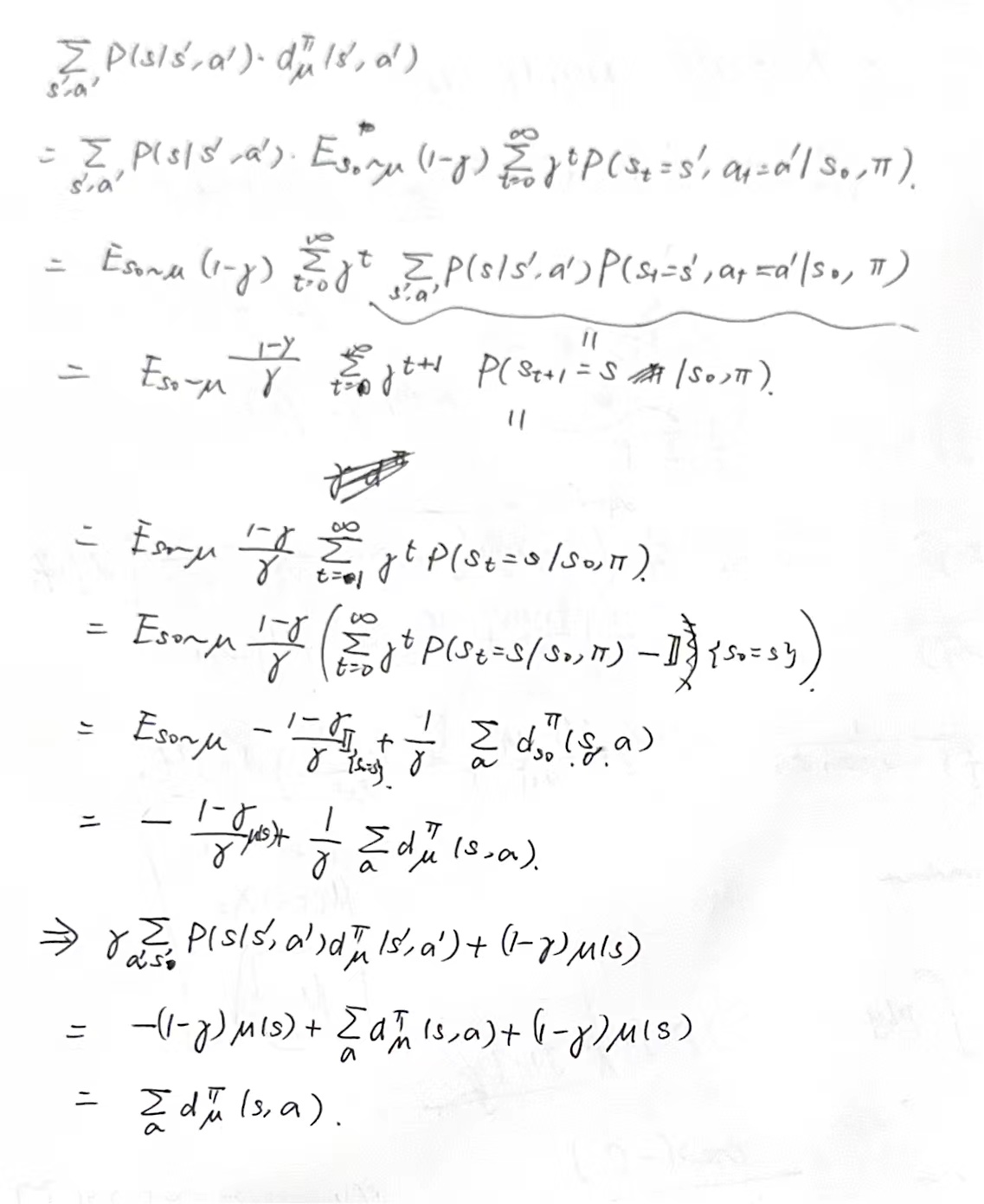
Dual LP

For a fixed (possibly stochastic) policy $\pi$$\pi$, let us define a visitation measure over states and actions induced by following $\pi$$\pi$ after starting at $s_0$$s_0$. Precisely, define this distribution, $d_{s_0}^{\pi },$$d^{\pi}_{s_0},$ as follows:

where $\stackrel{\pi }{Pr}(s_t=s,a_t=a|s_0)$$\Pr^{\pi}(s_t=s,a_t=a|s_0)$ is the probability that $s_t=s$$s_t=s$ and $a_t=a,$$a_t=a,$ after starting at state $s_0$$s_0$ and following $\pi$$\pi$ thereafter. It is straightforward to verify that $d_{s_0}^{\pi }$$d^\pi_{s_0}$ is a distribution over $\mathcal{S}\times \mathcal{A}.$$\mathcal{S}\times\mathcal{A}.$ We also overload notation and write:

for a distribution $\mu$$\mu$ over $\mathcal{S}$$\mathcal S$. Recall Lemma 1.6 provides a way to easily compute $d_{\mu }^{\pi }(s,a)$$d_\mu^\pi(s,a)$ through an appropriate vector-matrix multiplication.

Remarks: Lemma 1.6 gives

Thus, actually we have

and

It is straightforward to verify that $d_{\mu }^{\pi }$$d_\mu^\pi$ satisfies, for all states $s\in \mathcal{S}$$s\in\mathcal{S}$

Remarks: Simply we have

Let us define the state-action polytope as follows:

We now see that this set precisely characterizes all state-action visitation distributions.

Proposition 1.15. We have that ${\mathcal{K}}_{\mu }$$\mathcal{K}_\mu$ is equal to the set of all feasible state-action distributions, i.e. $d\in {\mathcal{K}}_{\mu }$$d \in \mathcal K_\mu$, if and only if there exists a stationary (and possibly randomized) policy $\pi$$\pi$ such that $d_{\mu }^{\pi }=d$$d_\mu^\pi=d$.

With respect the variables $d\in {\mathbb{R}}^{|\mathcal{S}|\cdot |\mathcal{A}|}$$d\in\mathbb{R}^{|\mathcal{S}|\cdot|\mathcal{A}|}$ , the dual LP formulation is as follows

If $d^{\star }$$d^\star$ is the solution to this LP, and provided that $\mu$$\mu$ has full support, then we have that:

is an optimal policy. An alternative optimal policy is $\arg max{d}^{\star }(s,a)$$\arg\max d^{\star}(s,a)$ (and these policies are identical if the optimal policy is unique).

Sample Complexity and Sampling Models

we are interested understanding the number of samples required to find a near optimal policy, i.e. the sample complexity.

A generative model provides us with a sample $s^{\prime }\sim P(·|s,a)$$s'\sim P(·|s,a)$ and the reward $r(s,a)$$r(s, a)$ upon input of a state action pair $(s,a)$$(s, a)$.

The offline RL setting. The offline RL setting is where the agent has access to an offline dataset, say generated under some policy (or a collection of policies). In the simplest of these settings, we may assume our dataset is of the form $\{(s,a,s^{\prime },r)\}$$\{(s,a,s',r)\}$ where $r$$r$ is the reward (corresponding to $r(s,a)$$r(s,a)$ if the reward is deterministic) and $s^{\prime }\sim P(\cdot |s,a).$$s'\sim P(\cdot|s,a).$ Furthermore, for simplicity it can be helpful to assume that the $(s,a)$$(s,a)$ pairs in this dataset were sampled i.i.d. from some fixed distribution $\nu$$\nu$ over $\mathcal{S}\times \mathcal{A}$$\mathcal{S}\times\mathcal{A}$.

Bonus: Advantages and The Performance Difference Lemma

The advantage $A^{\pi }(s,a)$$A^{\pi}(s,a)$ of a policy $\pi$$\pi$ is defined as

Note that:

for all state-action pairs.

Analogous to the state-action visitation distribution (see Equation 0.8), we can define a visitation measure over jus the states. When clear from context, we will overload notation and also denote this distribution by $d_{s_0}^{\pi },$$d^\pi_{s_0},$ where:

Here, $\stackrel{\pi }{Pr}(s_t=s|s_0)$$\Pr^{\pi}(s_t=s|s_0)$is the state visitation probability, under r starting at state so. Again, we write:

for a distribution $\mu$$\mu$ over $\mathcal{S}$$\mathcal S$.

Remarks: In Equation 0.8., we define $d_{s_0}^{\pi }(s,a):=(1-\gamma )\sum _{t=0}^{\mathrm{\infty }}{\gamma }^t\stackrel{\pi }{Pr}(s_t=s,a_t=a|s_0)$$d_{s_0}^{\pi}(s,a):=(1-\gamma)\sum\limits_{t=0}^{\infty}\gamma^t\Pr^{\pi}(s_t=s,a_t=a|s_0)$, so the only difference is in $a$$a$, such that $d_{s_0}^{\pi }(s)=\sum _a{d}_{s_0}^{\pi }(s,a)$$d_{s_0}^{\pi}(s) = \sum_a d_{s_0}^{\pi}(s,a)$.

Lemma 1.16.（The performance difference lemma) For all policies $\pi ,{\pi }^{\prime }$$\pi, \pi'$ and distributions $\mu$$\mu$ over $\mathcal{S}$$\mathcal S$,

Proof at P19 of the book