Overview

This is my note for Chapter 8 of Reinforcement Learning Theory.

Linearly Parameterized MDPs

The whole idea is similar to Chapter 6, where we extend from MAB to linear bandits to deal with a huge action space. We seek some sort of extension to discrete MDPs in Chapter 6.

Setting

Setting is similar to Chapter 7, i.e., finite horizon+episodic setting+minimize regret

Low-Rank MDPs and Linear MDPs

Here $\mathcal{S}$$\mathcal S$ and $\mathcal{A}$$\mathcal A$ can be infinite. Without any further structural assumption, the lower bounds we saw in the Generalization Lecture forbid us to get a polynomial regret bound.

Remarks: Remind that in Chapter 7, we have $\tilde{O}(H^{2}S\sqrt{AK})$$\tilde{O}(H^2 S \sqrt{AK})$ regret bound for UCBVI. If $\mathcal{S}$$\mathcal S$ and $\mathcal{A}$$\mathcal A$ are infinite/continuous, This is obviously quite bad. Also remind that in Chapter 6, we have $\tilde{O}(d\sqrt{T})$$\tilde{O}(d\sqrt{T})$ regret bound for LinUCB (here $d$$d$ is dimension and $T$$T$ is iterations). We see the main motivation is that we need to impose some structural assumption, such that we can get a polynomial bound for regret.

The structural assumption we make in this note is a linear structure in both the reward and the transition.

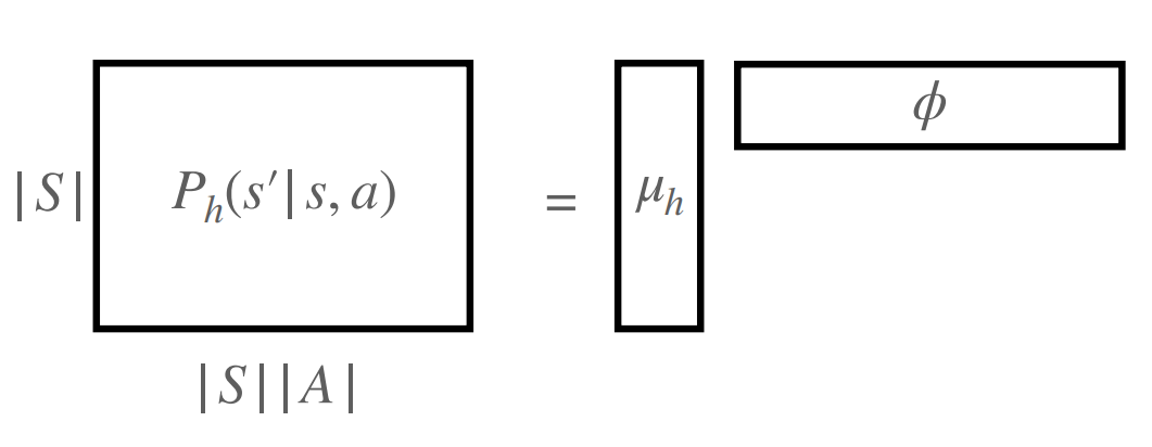
Definition 8.1 (Linear MDPs). Consider transition $\{P_h\}$$\{P_h\}$ and $\{r_h\}$$\{r_h\}$. A linear MDP has the following structures on $\{r_h\}$$\{r_h\}$ and $\{P_h\}$$\{P_h\}$:

where $\varphi$$\phi$ is a known state-action feature map $\varphi :\mathcal{S}\times \mathcal{A}\mapsto {\mathbb{R}}^d,$$\phi:\mathcal{S}\times\mathcal{A}\mapsto\mathbb{R}^d,$ and ${\mu }_h^{\star }\in {\mathbb{R}}^{|\mathcal{S}|\times d}.$$\mu_h^{\star}\in\mathbb{R}^{|\mathcal{S}|\times d}.$ Here $\varphi$$\phi$, ${\theta }_h^{\star }$$\theta^\star_h$ are known to the learner, while ${\mu }^{\star }$$\mu^\star$ is unknown. We further assume the following norm bound on the parameters:（1) $\underset{s,a}{sup}\parallel \varphi (s,a){\parallel }_2\le 1,$$\sup_{s,a}\|\phi(s,a)\|_2\le1,$ (2) $\parallel v^{\mathrm{\top }}{\mu }_h^{\star }{\parallel }_2\le \sqrt{d}$$\|v^\top\mu_h^\star\|_2\le\sqrt{d}$ for any $v$$v$ such that $\parallel v{\parallel }_{\mathrm{\infty }}\le 1$$\|v\|_\infty \leq 1$, and all $h$$h$, and (3) $\parallel {\theta }_h^{\star }{\parallel }_2\le W$$\|\theta^\star_h\|_2 \le W$ for all $h$$h$. We assume $r_h(s,a)\in [0,1]$$r_h(s,a)\in[0,1]$ for all $h$$h$ and $s,a$$s, a$.

The intuition of this assumption is that now we can have poly($d$$d$) instead of $|\mathcal{S}|$$|\mathcal S|$ or $|\mathcal{A}|$$|\mathcal A|$.

Remarks: The connection to tabular MDPs is that if $\varphi$$\phi$ is a one-hot mapping, then ${\mu }_h^{\star }\varphi (s,a)=({\mu }_h^{\star }{)}_i$$\mu_h^\star \phi(s, a) = (\mu_h^\star)_i$, where $({\mu }_h^{\star }{)}_i$$(\mu_h^\star)_i$ denotes the $i$$i$-th column vector and known reward $r_h(s,a)=[{\theta }_h^{\star }{]}_i$$r_h(s, a) = [\theta^\star_h]_i$. This reduces to tabular MDPs.

An example is latent variable models, see slides.

Remarks: Linear MDP = low-rank+known $\varphi$$\phi$.

Planning in Linear MDPs

An important observation in linear MDPs is the linearity of everything, i.e.,

where $\cdot$$\cdot$ denotes the inner product. And thus we can define ${\pi }^{\star }=\arg \underset{a}{max}{Q}_h^{\star }(s,a)$$\pi^\star = \arg \max_a Q^\star_h(s, a)$ and $V^{\star }(s)=\underset{a}{max}{Q}_h^{\star }(s,a)$$V^\star(s) = \max_a Q^\star_h(s, a)$. More generally, we have

Claim 8.2. Consider any arbitrary function $f:\mathcal{S}\mapsto [0,H].$$f:\mathcal{S}\mapsto[0,H].$ At any time step $h\in [0,\dots H-1]$$h \in [0,\ldots H-1]$ there must exist a $w\in {\mathbb{R}}^d$$w \in \mathbb{R}^d$, such that, for all $s,a\in \mathcal{S}\times \mathcal{A}:$$s,a \in \mathcal{S}\times \mathcal{A} \colon$

where $\mathcal{T}$$\mathcal T$ is the bellman operator.

Proof: derive by definition.

UCBVI?

1. Learn transmission model $\{{\hat{P}}_h^n{\}}_{h=0}^{H-1}$$\{\widehat{P}_h^n\}_{h=0}^{H-1}$ from all previous data $\{s_h^i,a_h^i,s_{h+1}^i{\}}_{i=0}^{n-1}$$\{s_h^i,a_h^i,s_{h+1}^i\}_{i=0}^{n-1}$

2. Design reward bonus $b_h^n(s,a),\mathrm{\forall }s,a$$b^n_h(s,a),\forall s,a$

3. Plan: ${\pi }^{n+1}=\text{Value-lter}(\{{\hat{P}}^n{\}}_h,\{r_h+b_h^n\})$$\pi^{n+1} = \text{Value-lter} \left(\{\widehat{P}^n\}_h,\{r_h+b_h^n\}\right)$

4. Execute for $H$$H$ steps

Remarks: We can see that the general framework is identical, so the point falls on how to design bonus and how to learn the transition kernel.

Learning Transition using Ridge Linear Regression

Remarks: Recall that in tabular MDPs, we use empirical estimation for transition. However, in this setting, this becomes infeasible as $|\mathcal{S}|$$|\mathcal S|$ and $|\mathcal{A}|$$|\mathcal A|$ are super big/continuous. So we need a way out.

In this section, we consider the following simple question: given a dataset of state-action-next state tuples, how can we learn the transition $P_h$$P_h$ for all $h$$h$?

We consider a particular episode $n$$n$. Similar to Tabular-UCBVI, we learn a model at the very beginning of episode $n$$n$ using all data from the previous episodes (episode $1$$1$ to the end of episode $n-1$$n-1$). We denote such dataset as:

We maintain the following statistics using $D_h^n$$D_h^n$:

Remarks: when $\varphi$$\phi$ is a one-hot mapping, the ${\mathrm{\Lambda }}_h^n$$\Lambda_h^n$ is a diagonal matrix with $N_h^n(s,a)$$N_h^n(s, a)$ as elements. (Remind that $N_h^n(s,a)=\sum _{i=0}^{n-1}\mathbb{I}\{(s_h^i,a_h^i)=(s,a)\}$$N_h^n(s, a) = \sum_{i=0}^{n-1} \mathbb{I}\{(s^i_h, a_h^i) = (s, a)\}$.)

Remarks: A bound: $|{\mathrm{\Lambda }}_h^n|=|\sum _{i=0}^{n-1}\varphi (s_h^i,a_h^i{)}^{\mathrm{\top }}\varphi (s_h^i,a_h^i)+\lambda I|\le |n+\lambda I|\le (n+\lambda {)}^d$$|\Lambda_h^n| = |\sum\limits_{i=0}^{n-1}\phi(s_h^i,a_h^i)^\top \phi(s_h^i,a_h^i)+\lambda I| \le |n + \lambda I| \le (n+\lambda)^d$. The interchange inside the determinant is simply due to $x^{\mathrm{\top }}x$$x^\top x$ and $x{x}^{\mathrm{\top }}$$xx^\top$ having the same non-zero eigenvalues.

We consider the following multi-variate linear regression problem. Denote $\delta (s)$$\delta(s)$ as a one-hot vector that has zero everywhere except that the entry corresponding to $s$$s$ is one. Denote ${ϵ}_h^i=P(\cdot \mid s_h^i,a_h^i)-\delta \left(s_{h+1}^i\right)$$\epsilon_h^i=P\left(\cdot \mid s_h^i, a_h^i\right)-\delta\left(s_{h+1}^i\right)$. Conditioned on history ${\mathcal{H}}_h^i$$\mathcal{H}_h^i$ (history ${\mathcal{H}}_h^i$$\mathcal{H}_h^i$ denotes all information from the very beginning of the learning process up to and including $(s_h^i,a_h^i))$$\left.\left(s_h^i, a_h^i\right)\right)$, we have:

simply because $s_{h+1}^i$$s_{h+1}^i$ is sampled from $P_h(\cdot \mid s_h^i,a_h^i)$$P_h\left(\cdot \mid s_h^i, a_h^i\right)$ conditioned on $(s_h^i,a_h^i)$$\left(s_h^i, a_h^i\right)$ (Remarks: In other words, $\mathbb{E}[\delta (s_{h+1}^i)|(s_h^i,a_h^i)]=P_h(\cdot |s_h^i,a_h^i)$$\mathbb E[\delta(s_{h+1}^i)|(s_h^i, a_h^i)] = P_h(\cdot | s_h^i, a_h^i)$). Also note that ${\Vert {ϵ}_h^i\Vert }_1\le 2$$\left\|\epsilon_h^i\right\|_1 \leq 2$ for all $h,i$$h, i$.

Since ${\mu }_h^{\star }\varphi (s_h^i,a_h^i)=P_h(\cdot \mid s_h^i,a_h^i)$$\mu_h^{\star} \phi\left(s_h^i, a_h^i\right)=P_h\left(\cdot \mid s_h^i, a_h^i\right)$, and $\delta \left(s_{h+1}^i\right)$$\delta\left(s_{h+1}^i\right)$ is an unbiased estimate of $P_h(\cdot \mid s_h^i,a_h^i)$$P_h\left(\cdot \mid s_h^i, a_h^i\right)$ conditioned on $s_h^i,a_h^i$$s_h^i, a_h^i$, it is reasonable to learn ${\mu }^{\star }$$\mu^{\star}$ via regression from $\varphi (s_h^i,a_h^i)$$\phi\left(s_h^i, a_h^i\right)$ to $\delta \left(s_{h+1}^i\right)$$\delta\left(s_{h+1}^i\right)$. This leads us to the following ridge linear regression:

Ridge linear regression has the following closed-form solution:

Note that ${\hat{\mu }}_h^n\in {\mathbb{R}}^{|\mathcal{S}|\times d}$$\widehat{\mu}_h^n \in \mathbb{R}^{|\mathcal{S}| \times d}$, so we never want to explicitly store it. Note that we will always use ${\hat{\mu }}_h^n$$\widehat{\mu}_h^n$ together with a specific $s,a$$s, a$ pair and a value function $V$$V$ (think about value iteration case), i.e., we care about ${\hat{P}}_h^n(\cdot \mid s,a)\cdot V:=({\hat{\mu }}_h^n\varphi (s,a))\cdot V$$\widehat{P}_h^n(\cdot \mid s, a) \cdot V:=\left(\widehat{\mu}_h^n \phi(s, a)\right) \cdot V$, which can be re-written as:

Thus we only need to compute ${\hat{P}}_h^n(\cdot \mid s,a)\cdot V$$\widehat{P}_h^n(\cdot \mid s, a) \cdot V$, which is simply poly($d,n$$d, n$), not depending on $|\mathcal{S}|$$|\mathcal S|$.

Lemma 8.3 (Difference between ${\hat{\mu }}_h$$\widehat{\mu}_h$ and ${\mu }_h^{\star }$$\mu_h^{\star}$ ). For all $n$$n$ and $h$$h$, we must have:

Proof: We start from the closed-form solution of ${\hat{\mu }}_h^n$$\widehat{\mu}_h^n$ :

Rearrange terms, we conclude the proof.

Lemma 8.4. Fix $V:\mathcal{S}\mapsto [0,H]$$V: \mathcal{S} \mapsto[0, H]$. For all $n$$n$ and $s,a\in \mathcal{S}\times \mathcal{A}$$s, a \in \mathcal{S} \times \mathcal{A}$, and $h$$h$, with probability at least $1-\delta$$1-\delta$, we have:

Proof: We first check the noise terms ${\left\{V^{\mathrm{\top }}{ϵ}_h^i\right\}}_{h,i}$$\left\{V^{\top} \epsilon_h^i\right\}_{h, i}$. Since $V$$V$ is independent of the data (it's a pre-fixed function), and by linear property of expectation, we have:

Hence, this is a Martingale difference sequence. Using the Self-Normalized vector-valued Martingale Bound (Lemma A.9), we have that for all $n$$n$, with probability at least $1-\delta$$1-\delta$ :

Apply union bound over all $h\in [H]$$h \in[H]$, we get that with probability at least $1-\delta$$1-\delta$, for all $n,h$$n, h$ :

Uniform Convergence via Covering

The reason to use covering here is that the function class is infinite.

Lemma 8.5. The $ϵ$$\epsilon$-covering number of the ball $\mathrm{\Theta }=\{\theta \in {\mathbb{R}}^d:\parallel \theta {\parallel }_2\le R\in {\mathbb{R}}^{+}\}$$\Theta=\left\{\theta \in \mathbb{R}^d:\|\theta\|_2 \leq R \in \mathbb{R}^{+}\right\}$is upper bounded by $(1+2R/ϵ{)}^d$$(1+2 R / \epsilon)^d$.

Proof: We already show this in Chapter 7. Refer to https://arxiv.org/pdf/1011.3027.pdf Lemma 5.2.

We can extend the above definition to a function class. Specifically, we look at the following function. For a triple of $(w,\beta ,\mathrm{\Lambda })$$(w, \beta, \Lambda)$ where $w\in {\mathbb{R}}^d$$w \in \mathbb{R}^d$ and $\parallel w{\parallel }_2\le L,\beta \in [0,B]$$\|w\|_2 \leq L, \beta \in[0, B]$, and $\mathrm{\Lambda }$$\Lambda$ such that ${\sigma }_{min}(\mathrm{\Lambda })\ge \lambda$$\sigma_{\min }(\Lambda) \geq \lambda$, we define $f_{w,\beta ,\mathrm{\Lambda }}:\mathcal{S}\mapsto [0,R]$$f_{w, \beta, \Lambda}: \mathcal{S} \mapsto[0, R]$ as follows:

We denote the function class $\mathcal{F}$$\mathcal{F}$ as:

Note that $\mathcal{F}$$\mathcal{F}$ contains infinitely many functions as the parameters are continuous. However we will show that it has finite covering number that scales exponentially with respect to the number of parameters in $(w,\beta ,\mathrm{\Lambda })$$(w, \beta, \Lambda)$.

Why do we look at $\mathcal{F}$$\mathcal{F}$ ? As we will see later in this chapter $\mathcal{F}$$\mathcal{F}$ contains all possible ${\hat{Q}}_h$$\widehat{Q}_h$ functions one could encounter during the learning process.

Lemma 8.6 ( $ϵ$$\epsilon$-covering dimension of $\mathcal{F})$$\mathcal{F})$. Consider $\mathcal{F}$$\mathcal{F}$ defined in Eq. 0.6. Denote its $ϵ$$\epsilon$-cover as ${\mathcal{N}}_{ϵ}$$\mathcal{N}_\epsilon$ with the ${\ell }_{\mathrm{\infty }}$$\ell_{\infty}$ norm as the distance metric, i.e., $d(f_1,f_2)={\Vert f_1-f_2\Vert }_{\mathrm{\infty }}$$d\left(f_1, f_2\right)=\left\|f_1-f_2\right\|_{\infty}$ for any $f_1,f_2\in \mathcal{F}$$f_1, f_2 \in \mathcal{F}$. We have that:

Note that the $ϵ$$\epsilon$-covering dimension scales quadratically with respect to $d$$d$.

Proof: We start from building a net over the parameter space $(w,\beta ,\mathrm{\Lambda })$$(w, \beta, \Lambda)$, and then we convert the net over parameter space to an $ϵ$$\epsilon$-net over $\mathcal{F}$$\mathcal{F}$ under the ${\ell }_{\mathrm{\infty }}$$\ell_{\infty}$ distance metric.

We pick two functions that corresponding to parameters $(w,\beta ,\mathrm{\Lambda })$$(w, \beta, \Lambda)$ and $(\hat{w},\hat{\beta },\hat{\mathrm{\Lambda }})$$(\hat{w}, \hat{\beta}, \widehat{\Lambda})$.

Remarks: Assume $\underset{a}{max}f(a)-\underset{a}{max}g(a)\ge 0$$\max_a f(a) - \max_a g(a) \ge 0$, then $|\underset{a}{max}f(a)-\underset{a}{max}g(a)|\le \underset{a}{max}f(a)-g(a_0),\mathrm{\forall }{a}_0$$|\max_a f(a) - \max_a g(a)| \le \max_a f(a) - g(a_0), \forall a_0$. Thus we have $|\underset{a}{max}f(a)-\underset{a}{max}g(a)|\le \underset{a}{max}|f(a)-g(a)|$$|\max_a f(a) - \max_ag(a)| \le \max_a|f(a) - g(a)|$.

Remarks: The forth line is due to the assumption that $\parallel \varphi {\parallel }_{\mathrm{\infty }}\le 1$$\|\phi\|_\infty \le 1$.

Note that ${\mathrm{\Lambda }}^{-1}$$\Lambda^{-1}$ is a PD matrix with ${\sigma }_{max}\left({\mathrm{\Lambda }}^{-1}\right)\le 1/\lambda$$\sigma_{\max }\left(\Lambda^{-1}\right) \leq 1 / \lambda$. Now we consider the $ϵ/3$$\epsilon / 3$-Net ${\mathcal{N}}_{ϵ/3,w}$$\mathcal{N}_{\epsilon / 3, w}$ over $\{w:\parallel w{\parallel }_2\le L\},\sqrt{\lambda }ϵ/3$$\left\{w:\|w\|_2 \leq L\right\}, \sqrt{\lambda} \epsilon / 3$-net ${\mathcal{N}}_{\sqrt{\lambda }ϵ/3,\beta }$$\mathcal{N}_{\sqrt{\lambda} \epsilon / 3, \beta}$ over interval $[0,B]$$[0, B]$ for $\beta$$\beta$, and ${ϵ}^2/\left(9B^2\right)$$\epsilon^2 /\left(9 B^2\right)$-net ${\mathcal{N}}_{{ϵ}^2/(9B),\mathrm{\Lambda }}$$\mathcal{N}_{\epsilon^2 /(9 B), \Lambda}$ over $\{\mathrm{\Lambda }:\parallel \mathrm{\Lambda }{\parallel }_F\le \sqrt{d}/\lambda \}$$\left\{\Lambda:\|\Lambda\|_F \leq \sqrt{d} / \lambda\right\}$.

Remarks: This is just the $ϵ/3$$\epsilon /3$ method, covering net version.

The product of these three nets provide a $ϵ$$\epsilon$-cover for $\mathcal{F}$$\mathcal{F}$, which means that that size of the $ϵ$$\epsilon$-net ${\mathcal{N}}_{ϵ}$$\mathcal{N}_\epsilon$ for $\mathcal{F}$$\mathcal{F}$ is upper bounded as:

Now we can build a uniform convergence argument for all $f\in \mathcal{F}$$f \in \mathcal{F}$. Yeyah :) ! Lemma 8.7 (Uniform Convergence Results). Set $\lambda =1$$\lambda=1$. Fix $\delta \in (0,1)$$\delta \in(0,1)$. For all $n,h$$n, h$, all $s,a$$s, a$, and all $f\in \mathcal{F}$$f \in \mathcal{F}$, with probability at least $1-\delta$$1-\delta$, we have:

Proof: Recall Lemma 8.4 , we have with probability at least $1-\delta$$1-\delta$, for all $n,h$$n, h$, for a pre-fixed $V$$V$ (independent of the random process):

where we have used the fact that $\parallel \varphi {\parallel }_2\le 1,\lambda =1$$\|\phi\|_2 \leq 1, \lambda=1$, and ${\Vert {\mathrm{\Lambda }}_h^n\Vert }_2\le N+1$$\left\|\Lambda_h^n\right\|_2 \leq N+1$.

Remarks: $N$$N$ is the total number of episodes. Note that $\det ({\mathrm{\Lambda }}_h^n{)}^{1/2}\det (\lambda I{)}^{-1/2}\le (n+\lambda {)}^{d/2}{\lambda }^{-d/2}\le (N/\lambda +1{)}^{d/2}=(N+1{)}^{d/2}$$\operatorname{det}(\Lambda_h^n)^{1 / 2} \operatorname{det}(\lambda I)^{-1 / 2} \le (n + \lambda)^{d/2} \lambda^{-d/2} \le (N/\lambda + 1)^{d/2} = (N+1)^{d/2}$.

Denote the $ϵ$$\epsilon$-cover of $\mathcal{F}$$\mathcal{F}$ as ${\mathcal{N}}_{ϵ}$$\mathcal{N}_\epsilon$. With an application of a union bound over all functions in ${\mathcal{N}}_{ϵ}$$\mathcal{N}_\epsilon$, we have that with probability at least $1-\delta$$1-\delta$, for all $V\in {\mathcal{N}}_{ϵ}$$V \in \mathcal{N}_\epsilon$, all $n,h$$n, h$, we have:

Recall Lemma 8.6, substitute the expression of $\ln \left|{\mathcal{N}}_{ϵ}\right|$$\ln \left|\mathcal{N}_\epsilon\right|$ into the above inequality, we get:

Now consider an arbitrary $f\in \mathcal{F}$$f \in \mathcal{F}$. By the definition of $ϵ$$\epsilon$-cover, we know that for $f$$f$, there exists a $V\in {\mathcal{N}}_{ϵ}$$V \in \mathcal{N}_\epsilon$, such that $\parallel f-V{\parallel }_{\mathrm{\infty }}\le ϵ$$\|f-V\|_{\infty} \leq \epsilon$. Thus, we have:

where in the second inequality we use the fact that ${\Vert \sum _{i=1}^{n-1}\varphi (s_h^i,a_h^i)(V-f{)}^{\mathrm{\top }}{ϵ}_h^i\Vert }_{{\left({\mathrm{\Lambda }}_h^n\right)}^{-1}}^2\le 4{ϵ}^{2}N$$\left\|\sum_{i=1}^{n-1} \phi\left(s_h^i, a_h^i\right)(V-f)^{\top} \epsilon_h^i\right\|_{\left(\Lambda_h^n\right)^{-1}}^2 \leq 4 \epsilon^2 N$, which is from

Remarks: Remind that ${\Vert {ϵ}_h^i\Vert }_1\le 2$$\left\|\epsilon_h^i\right\|_1 \leq 2$, which gives $(V-f{)}^{\mathrm{\top }}{ϵ}_h^i\le \parallel V-f{\parallel }_{\mathrm{\infty }}\parallel {ϵ}_h^i{\parallel }_1\le 2ϵ$$(V-f)^\top \epsilon_h^i \le \|V-f\|_\infty \|\epsilon_h^i\|_1 \le 2\epsilon$.

Set $ϵ=1/\sqrt{N}$$\epsilon=1 / \sqrt{N}$, we get:

where we recall $\lesssim$$\lesssim$ ignores absolute constants. Now recall that we can express $({\hat{P}}_h^n(\cdot \mid s,a)-P(\cdot \mid s,a))\cdot f=\varphi (s,a{)}^{\mathrm{\top }}{({\hat{\mu }}_h^n-{\mu }_h^{\star })}^{\mathrm{\top }}f$$\left(\widehat{P}_h^n(\cdot \mid s, a)-P(\cdot \mid s, a)\right) \cdot f=\phi(s, a)^{\top}\left(\widehat{\mu}_h^n-\mu_h^{\star}\right)^{\top} f$. Recall Lemma 8.3, we have:

Remarks: For the second inequality, we have $|\lambda \varphi (s,a{)}^{\mathrm{\top }}{\left({\mathrm{\Lambda }}_h^n\right)}^{-1}{\left({\mu }_h^{\star }\right)}^{\mathrm{\top }}f|=|\varphi (s,a{)}^{\mathrm{\top }}{\left({\mathrm{\Lambda }}_h^n\right)}^{-1/2}{\left({\mathrm{\Lambda }}_h^n\right)}^{-1/2}{\left({\mu }_h^{\star }\right)}^{\mathrm{\top }}f|\le {\Vert \varphi (s,a{)}^{\mathrm{\top }}{\left({\mathrm{\Lambda }}_h^n\right)}^{-1/2}\Vert }_2{\Vert {\left({\mathrm{\Lambda }}_h^n\right)}^{-1/2}{\left({\mu }_h^{\star }\right)}^{\mathrm{\top }}f\Vert }_2=\parallel \varphi (s,a){\parallel }_{{\left({\mathrm{\Lambda }}_h^n\right)}^{-1}}\parallel {\left({\mu }_h^{\star }\right)}^{\mathrm{\top }}f{\parallel }_{{\left({\mathrm{\Lambda }}_h^n\right)}^{-1}}$$\left|\lambda \phi(s, a)^{\top}\left(\Lambda_h^n\right)^{-1}\left(\mu_h^{\star}\right)^{\top} f\right| = \left| \phi(s, a)^{\top}\left(\Lambda_h^n\right)^{-1/2}\left(\Lambda_h^n\right)^{-1/2}\left(\mu_h^{\star}\right)^{\top} f\right| \le \left\| \phi(s, a)^{\top}\left(\Lambda_h^n\right)^{-1/2} \right\|_2 \left\| \left(\Lambda_h^n\right)^{-1/2} \left(\mu_h^{\star}\right)^{\top} f\right\|_2 = \|\phi(s, a)\|_{\left(\Lambda_h^n\right)^{-1}} \|\left(\mu_h^{\star}\right)^{\top} f\|_{\left(\Lambda_h^n\right)^{-1}}$ . Note that since $f\in \mathcal{F}$$f \in \mathcal F$, thus $\parallel f{\parallel }_{\mathrm{\infty }}\le H$$\|f\|_\infty \le H$, and assumption 2 yields $\parallel {\left({\mu }_h^{\star }\right)}^{\mathrm{\top }}f{\parallel }_{{\left({\mathrm{\Lambda }}_h^n\right)}^{-1}}\le \parallel {\left({\mathrm{\Lambda }}_h^n\right)}^{-1/2}{\parallel }_2\parallel {\left({\mu }_h^{\star }\right)}^{\mathrm{\top }}f{\parallel }_2\le H\sqrt{d}/\sqrt{\lambda }$$\|\left(\mu_h^{\star}\right)^{\top} f\|_{\left(\Lambda_h^n\right)^{-1}} \le \| \left(\Lambda_h^n\right)^{-1/2} \|_2\| \left(\mu_h^{\star}\right)^{\top} f\|_2 \le H \sqrt{d} / \sqrt{\lambda}$. (Note that the smallest eigenvalue of ${\mathrm{\Lambda }}_h^n\ge \lambda$$\Lambda_h^n \ge \lambda$.) Since $\lambda =1$$\lambda=1$, we obtain the first part of the second inequality. The second part is similar.

Remarks: Note that this is $\tilde{O}(Hd)\parallel \varphi (s,a){\parallel }_{({\mathrm{\Lambda }}_h^n{)}^{-1}}$$\tilde{O}(Hd) \|\phi(s, a)\|_{(\Lambda_h^n)^{-1}}$, which will be our bonus term.

Algorithm

Our algorithm, Upper Confidence Bound Value Iteration (UCB-VI) will use reward bonus to ensure optimism. Specifically, we will the following reward bonus, which is motivated from the reward bonus used in linear bandit:

where $\beta$$\beta$ contains poly of $H$$H$ and $d$$d$, and other constants and log terms ($\tilde{O}(Hd)$$\tilde{O}(Hd)$). Again to gain intuition, please think about what this bonus would look like when we specialize linear MDP to tabular MDP.

Algorithm 6 UCBVI for Linear MDPs

1. Input: parameters $\beta ,\lambda$$\beta, \lambda$

2. for $n=1\dots N$$n=1 \ldots N$ do

3. Compute ${\hat{P}}_h^n$$\widehat{P}_h^n$ for all $h$$h$ (Eq. 0.3)

4. Compute reward bonus $b_h^n$$b_h^n$ for all $h$$h$ (Eq. 0.7)

5. Run Value-Iteration on ${\{{\hat{P}}_h^n,r_h+b_h^n\}}_{h=0}^{H-1}$$\left\{\widehat{P}_h^n, r_h+b_h^n\right\}_{h=0}^{H-1}$ (Eq. 0.8)

6. Set ${\pi }^n$$\pi^n$ as the returned policy of VI.

7. end for

With the above setup, now we describe the algorithm. Every episode $n$$n$, we learn the model ${\hat{\mu }}_h^n$$\widehat{\mu}_h^n$ via ridge linear regression. We then form the quadratic reward bonus as shown in Eq. 0.7. With that, we can perform the following truncated Value Iteration (always truncate the $\mathrm{Q}$$\mathrm{Q}$ function at $H$$H$ ):

Note that above ${\hat{Q}}_h^n$$\widehat{Q}_h^n$ contains two components: a quadratic component and a linear component (w.r.t. $\varphi (s,a)$$\phi(s,a)$). And ${\hat{V}}_h^n$$\widehat{V}_h^n$ has the format of $f_{w,\beta ,\mathrm{\Lambda }}$$f_{w, \beta, \Lambda}$ defined in Eq. 0.5.

Now we show that ${\hat{V}}_h^n$$\widehat{V}_h^n$ falls into the category of $\mathcal{F}$$\mathcal F$:

Lemma 8.8. Assume $\beta \in [0,B]$$\beta \in[0, B]$. For all $n,h$$n, h$, we have ${\hat{V}}_h^n$$\widehat{V}_h^n$ is in the form of Eq. 0.5, and ${\hat{V}}_h^n$$\widehat{V}_h^n$ falls into the following class:

Proof: We just need to show that ${\theta }^{\star }+{\left({\hat{\mu }}_h^n\right)}^{\mathrm{\top }}{\hat{V}}_{h+1}^n$$\theta^{\star}+\left(\widehat{\mu}_h^n\right)^{\top} \widehat{V}_{h+1}^n$ has its ${\ell }_2$$\ell_2$ norm bounded. This is easy to show as we always have ${\Vert {\hat{V}}_{h+1}^n\Vert }_{\mathrm{\infty }}\le H$$\left\|\widehat{V}_{h+1}^n\right\|_{\infty} \leq H$ as we do truncation at Value Iteration:

Remarks: This is from assumption 3.

Now we use the closed-form of ${\hat{\mu }}_h^n$$\widehat{\mu}_h^n$ from Eq. 0.3:

where we use the fact that ${\Vert {\hat{V}}_{h+1}^n\Vert }_{\mathrm{\infty }}\le H,{\sigma }_{max}\left({\mathrm{\Lambda }}^{-1}\right)\le 1/\lambda$$\left\|\widehat{V}_{h+1}^n\right\|_{\infty} \leq H, \sigma_{\max }\left(\Lambda^{-1}\right) \leq 1 / \lambda$, and $\underset{s,a}{sup}\parallel \varphi (s,a){\parallel }_2\le 1$$\sup _{s, a}\|\phi(s, a)\|_2 \leq 1$

Analysis of UCBVI for Linear MDPs

We finally arrive at regret bound!!

In this section, we prove the following regret bound for UCBVI. Theorem 8.9 (Regret Bound). Set $\beta =\tilde{O}(Hd),\lambda =1$$\beta=\widetilde{O}(H d), \lambda=1$. UCBVI (Algorithm 6) achieves the following regret bound:

The main steps of the proof are similar to the main steps of UCBVI in tabular MDPs. We first prove optimism via induction, and then we use optimism to upper bound per-episode regret. Finally, we use simulation lemma to decompose the per-episode regret. In this section, to make notation simple, we set $\lambda =1$$\lambda=1$ directly.

Proving Optimism

Here we use a different $\beta$$\beta$, as the function class is slightly different from the one we use in Lemma 8.7. Check P93 of the book. We denote the event of Lemma 8.7 with ${\mathcal{E}}_{\text{model}}$$\mathcal E_{\text {model}}$.

Lemma 8.10 (Optimism). Assume event ${\mathcal{E}}_{\text{model }}$$\mathcal{E}_{\text {model }}$ is true. for all $n$$n$ and $h$$h$,

Proof: We consider a fixed episode $n$$n$. We prove via induction. Assume that ${\hat{V}}_{h+1}^n(s)\ge V_{h+1}^{\star }(s)$$\widehat{V}_{h+1}^n(s) \geq V_{h+1}^{\star}(s)$ for all $s$$s$. For time step $h$$h$, we have: